Introduction
Eigencircles are a concept I came across on this math stackexchange forum. They are a visualization of 2x2 matrices that provide a fascinating geometric understanding of matrix properties and their connection to eigenvectors and eigenvalues. I aim to summarize my understanding of eigencircles in this article.
What are Eigencircles?
An eigenvalue of a square matrix is a number such that for any non-zero vector . Let and . Then we can write this as
Now in the original article, Englefield and Farr state that matrices of the form are isomorphic to the reals under matrix addition and multiplication. They then utilize the field isomorphism
to rewrite as
After skimming through a few articles on abstract algebra, this made sense. But I came across another approach to arrive at that felt more intuitive. I describe this next.
From the SVD decomposition of a matrix, we know that every linear transformation represented by the matrix can be written as where are othgonal matrices and is a diagonal matrix. For the 2x2 case, the only orthogonal matrices are rotation and refelction matrices while the diagonal matrix is just a scaling matrix. Therefore, the 2x2 matrix simply rotates and scales every vector it is applied to. Notice that reflecting a vector along some axis of rotation can be expressed as a rotation.
In other words, for any vector , results in a rotation by angle and a scaling by factor . More formally, we can write this as
We can rewrite the matrix on the right hand side of the equality to be more succint
Now you may notice that this deviates from in that the minus signs on are reversed. This is the same as reversing the positive direction of the angles. Notice that
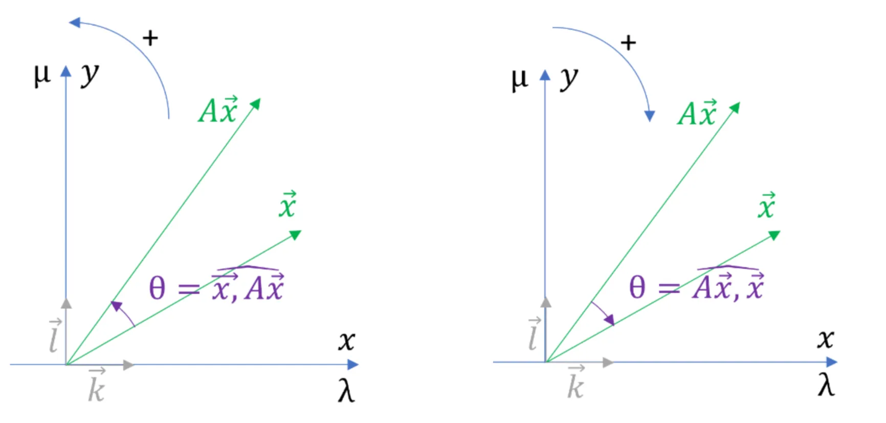
Figure 1: Taken from https://eigencircles.heavisidesdinner.com/eigenC/eigenC_book.html
In Figure 1, the left diagram corresponds to the case where we take and the right corresponds to the case where we consider . Therefore, it is equivalant to continue using either of the derivations. I will continue using .
Following the general procedure to determine eigenvalues but using the matrix specified in the RHS of (2), we get
This results in the following equation:
or, equivalently
Notice that is just . Now we define
Using to simplify we get
which is
where . gives the equation for the eigencircle of .
Deriving matrix properties from Eigencircles
Okay, now consider again. We know that the determinant of any matrix with a zero row or a zero column is zero. Considering the values of that would produce zero rows and columns, we get the following points: . These points must be on the eigencircle since they satisfy . Moreover, since the center of our eigencircle is defined to be the midpoint of and
these points define a rectangle.
Defining the points , we get the following graph.
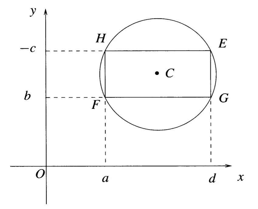
Before moving forward, you may notice the axes on Figure 2 corresponding to - these diagrams are from the original article and I was too lazy to refactor them. For the purposes of this article, and .
This visualization has some very interesting properties. Firstly, notice that if lies on the circle, then is an eigenvalue of . Let , then the vector is the corresponding eigenvector for .
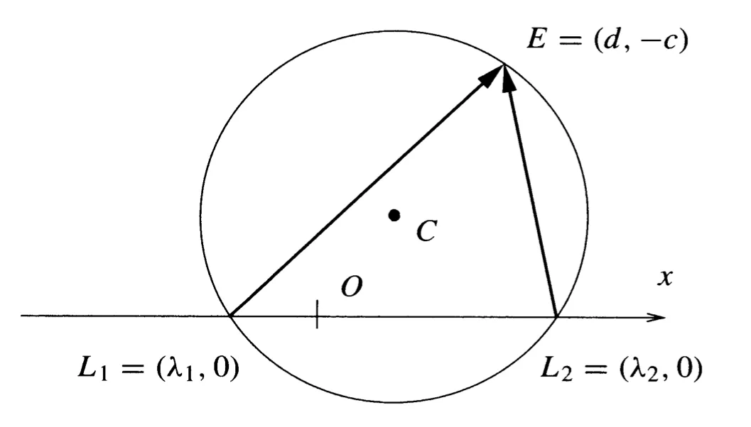
Figure 3: Determining eigenvectors from eigencircles
To see why, note that the vector . If this is an eigenvector corresponding to eigenvalue , then it must be in the nullspace of the matrix .
Let’s see if this is the case:
But we know that from (since lies on the eigencircle). Therefore, is indeed an eigenvector correspoinding to .
We can also use the eigencircle to prove that the product of eigenvalues for a 2x2 matrix is equal to the value of its determinant. We use the “power of a point” theorem to show this. The power of any point given by with respect to some circle with center is defined as
Geometrically, the power of a point states that “[if some] line through any point meets a circle in points and , the product of the lengths, and , is the same for any direction of the line. The lengths are signed, so the product is positive (negative) when is outside (inside) the circle.”
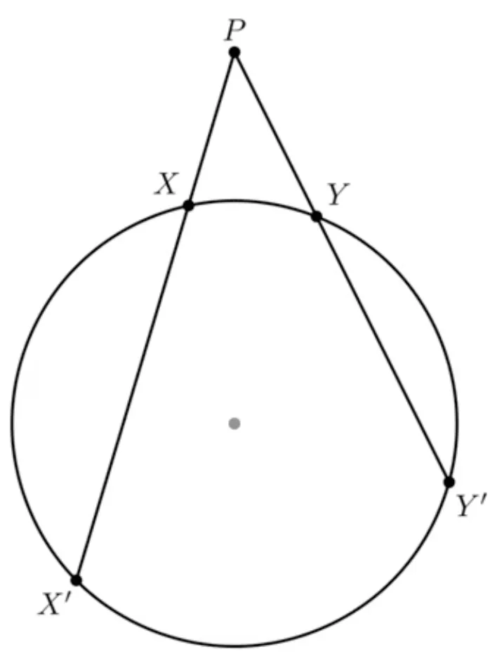
Figure 4: Power of a point theorem
Consider Figure 4. What the power of a point theorem says is that the (signed) product of the lengths . For more on the power of a point, refer to this link.
Consider . For the eigencircle, we can rewrite this as . Notice that this expression can be expressed as the LHS of by construction. So we get that the power of a point with respect to a eigencircle is given by
If we choose , we get that ! From Figure 3, we know that the (signed) lengths of the line segments and specify the eigenvalues. Well, from the power of a point theorem, we know that . Personally, I found this fascinating.
Finally, I am going to describe how the eigencircle relates to complex eigenvalues. Consider Figure 5a.
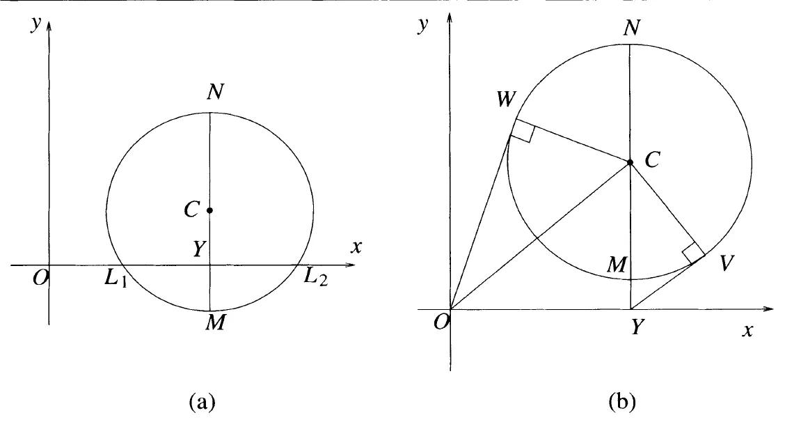
Figure 5: Eigencircles and complex eigenvalues
From the power of a point theorem, we know that the power of is given by
As , we have that (remember that we consider signed lengths). Knowing this, we can express the eigenvalues () in the following form
Now this is also valid for cases where the x-axis does not intersect the eigencircles (we will see why in a minute). Consider Figure 5b. We see that the quantity is now positive, there the value inside the square in is negative, giving us a complex value. If is a tangent to the circle at , then, by the power of a point theorem, we have that . Hence, we get the complex eigenvalues
Okay, so why is true when the x-axis does not intersect the eigencircle? Let’s figure out the coordinates . Well, we can see that (recall definitions ). Plugging this into we get
or equivalently,
Notice that if the x-axis does not intersect the eigencircle, then we have that and therefore , just as we had derived earlier. For this case, we need to realize that is undefined and we need to factor out the . More on this below.
For to be an eigenvalue, we know that equation must be satisfied for . Notice that equation can be rewritten as
This is just with the moved to the LHS. Plugging in , we get
as required. Therefore, you can determine all (both real and complex) eigenvalues using the eigencircle.
Visualizing the eigenvectors corresponding to complex eigenvalues would require an additional axis to account for the imaginary value. Let where . Consider Figure 6.
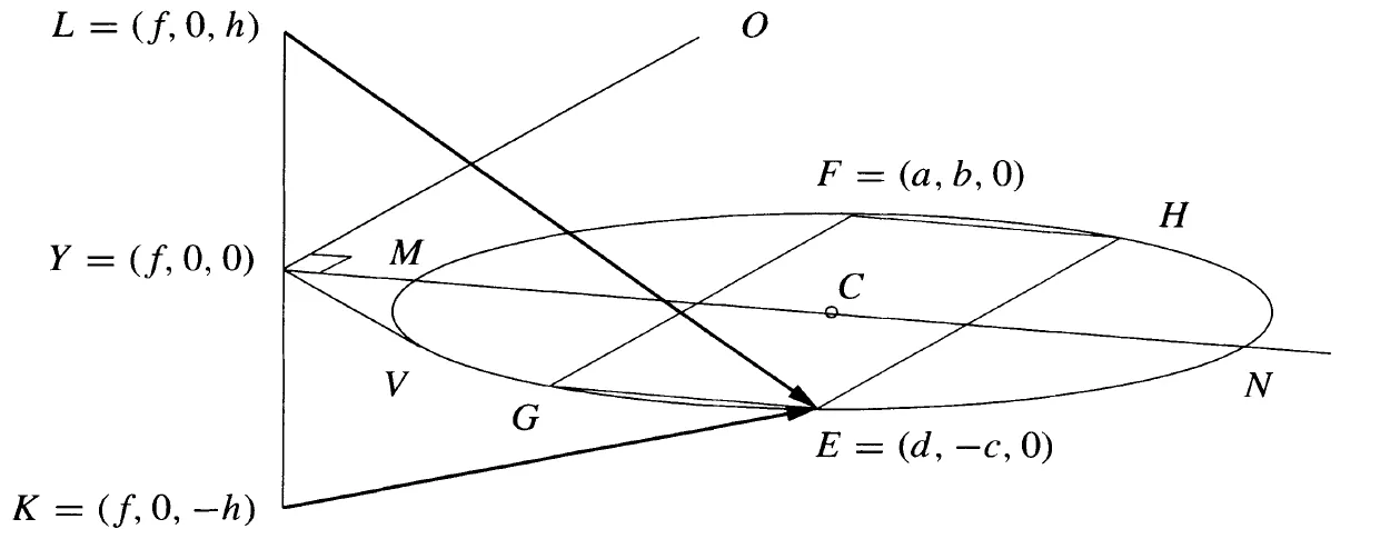
Figure 6: Geometric representation of complex eigenvectors
and
represent the complex eigenvectors. Notice
represents the complex eigenvector .
I am going to stop there. It was fun reading about eigencircles. I believe the way in which the properties of eigenvectors and eigenvalues expressed themselves through geometry was beautiful. Refer to [1] and [2] for the original articles on eigencircles.
References
- Englefield, M. J., & Farr, G. E. (2006). Eigencircles of 2 x 2 Matrices. Mathematics Magazine Vol. 79 Oct.,2006, 281-289.
- Englefield, M. J., & Farr, G. E. (2010). Eigencircles and associated surfaces. The Mathematical Gazette Vol.94 No. 531 (November 2010), 438-449.