Notes on Purely Functional Data Structures

Chapter 1: Introduction;

Chapter 2: Persistence

• In functional languages, you get “persistence” for free

• Persistance breaks amortized analyses
  • Amortized analysis
• Strict languages are clearly superior to lazy languages in at least one regard: analyzing runtimes, since in lazy languages, it is very, very hard to determine if a piece will ever be run

This book is about the fact that, even though immutability and other functional features may seem limiting, it is possible for purely functional data structures to be as efficient (asymptotically) as their mutable counterparts. Furthermore:

was incompatible with persistence [DST94, Ram92]. However, we show that memoization, in the form of lazy evaluation, is the key to reconciling the two.

Chapter 3: Some Familiar Data Structures in a Functional Setting

TODO

Chapter 4: Lazy Evalutation and $-notation

Supporting lazy evaluation in a strict language involves the addition of two primitives: - Delay - Force

• Wrapping calls with delay/force is very verbose, so this chapter introduces a more succint, neater $-based syntax
• Prepending an expression with $ will suspend it - $ parses as far to the right as possible – you can nest suspensions – $$e
• The $-notation is integration with pattern matching as well - avoiding the need for nested case expressions

Example (ML-esque pseudocode):

integer, T stream => T stream
fun take(n, s) =
	delay(fn () => case n of 
					0 => Nil
					_ => case (force s) of
						Nil => Nil
						| Cons(x, s') => Cons(x, take(n - 1, s')))

Now, using the neater $ integration with pattern matching (matching against a pattern prepended with $ will first force the expression and then match against the stuff after the $):

integer, T stream -> T stream
fun take(n, s) = $case (n, s) of  -- note the $ before case, the result type is a stream so this is necessary
					(0, _) => Nil
					(_, $Nil) => Nil
					(_, $Cons(x, s')) => Cons(x, take(n-1, s'))

integer, T stream -> T stream
fun take(n, s) = $Nil 
| take(_, $Nil) = $Nil
| take(_, $Cons(x, s')) = $Cons(x, take(n - 1, s'))

An example of this behaviour can be expressed by the append function on lazy list and streams:

For lazy lists:

fun s ++ t = $(force s @ force t)

^ when this is force, the entire computation is performed.

And for streams:

t stream, t stream -> t stream
fun s ++ t = $case s of 
			$Nil => force t
			| $Cons(x, s') => Cons(x, s' ++ t)

^ when this is forced, only the first step in the computation of appending the streams is performed.

Chapter 5: Fundamentals of Amortization

When proving amortization bounds, you prove that at any stage in the computation of this sequence, the accumulated amortized costs are less than the actual accumulated costs – the difference is called the accumulated savings.

Banker’s Method

Each operation has a cost, allocates “credits”, and spends credits.

\[ a_i = t_i + c_i + \bar{c_i}\] Each credit must be allocated before it is spent, i.e \(\sum{c_i} \geq \sum{\bar{c_i}}\) Proofs using this method need to show that the invariant above is maintained at every stage of the computation.

Physicist’s Method

• Define a potential function \(\Phi\) that assigns, to each state (i.e the state of objects in the internal representation of the data structure, after an operation is applied) a “potential” that represents a lower bound on the accumulated savings. There, the amortized cost after some step is defined to be: \[ a_i = t_i + \Phi(d_i) - \Phi(d_{i-1})\] where \(d_i\) and \(d_{i-1}\) are outputs of step i, i-1 repsectively.
• Typically, the potential function \(\Phi\) so that it is intially zero and always non-negative

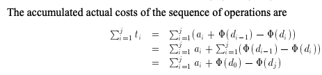
because the potential form a “telescoping series” (i.e same value alternating signs)

Example: Queues

• Queue are often implemented as a pair of lists, F and R
• The three main operations on a queue are:
  • head: get the first element
  • tail: drop the first element
  • snoc: append an element to the rear of the queue (snoc == cons to the right)

fun head(Queue {F = x::f, R = r}) = x

fun tail(Queue {F = [x], R = r}) = Queue {F = rev r, R = []}
	| tail(Queue {F = x::f, R = r}) = Queue {F = f, R = r}
	
fun snoc(Queue {F = [],...}, x) = Queue {F = [x], R = []}
	| snoc(Queue {F = f, R = r}, x) = Queue {F = f, R = x::r}

^ not including error handling

The invariant in this implementation is that F can only ever be empty if R is also empty. This means that, when tailing the queue, if F is a single element list, it gets replaced by the reverse of R (since R stores the rear of the queue _in reverse order, in order to support O(1) append)

• Using the banker’s method We define the credit invariant that the list R always has a number of credits equivalent to its length. snoc calls on non-empty queues have an amortized cost of two now, since they allocate one credit to the R list. All other operations take 1 step, except the tail calls that reverse the R list – which take m+1 steps, and spend the m credits, resulting in an amortized cost of 1!

• Using the physicist’s method Same idea, the potential function is the length of the rear list.

Note that, even though the proofs are nearly identical here, the physicist’s method is almost always simpler since all we need to do is define the potential function and then calculate. In the banker’s method, on the other hand, we need to define how many credits does each operation allocate and what the credit invariant is. Note that there are infinitely many valid credit assignments that maintain a given credit invariant, which just adds to the confusion.

Chapter 6: Amortization and Persistence via Lazy Evaluation

TODO